
I recently returned from the first star party of the season, and the first time I’ve done any astrophotography for more than 6 months. Hopefully, I’ll have a couple of images ready for you soon.
This edition of Pro Tips will explore some details of how Power*Star displays useful information. The embedded processor in P*S spends most of its time monitoring and reporting system status and faults. The P*S app queries this status frequently and provides a wealth of information for the user.
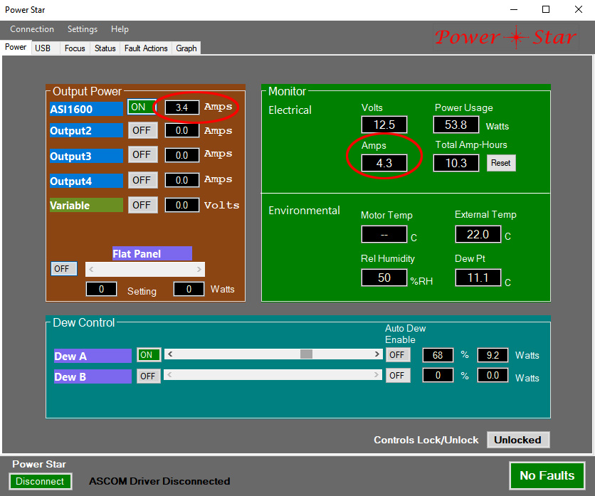
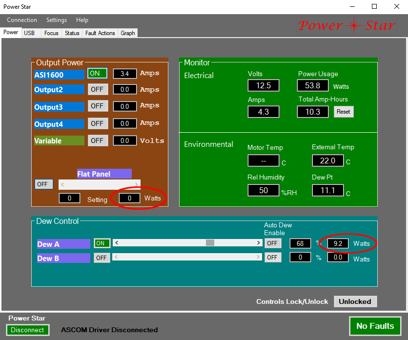
Perhaps the most important thing to understand is that the per-port current report is a direct measurement, but of limited accuracy. In particular, when the current is relatively low (less than 2 amps for ports 1 and 2, or less than 1 amp for all others) the accuracy declines significantly. The total current measurement is separate and different from the per-port measurements, and is much more accurate, despite its much larger range (up to 30 amps). Therefore, if you need a precise measurement of a device’s current draw it may be best to observe the total current display with the device on and off, then calculate the difference. Remember that the total current includes the USB ports and internal use (but devices connected to the pass-through PowerPole connector). The USB current is, of course, at 5V, not 12V. The voltage conversion happens with about 94% efficiency, so if a USB device is drawing 2 amps this will appear as approximately (2 * 5/12) / 0.94 = 0.89 amps, assuming the input voltage is exactly 12V. In the example below Output 1 (ASI1600) is drawing 3.4 amps, Dew Channel A is drawing an average of 9.2 watts, and the total current is 4.3 amps. The Input Voltage is 12.5V, so the average power use is 53.8 watts (4.3 * 12.5).
Current is measured for the dew heaters, but this value is not directly displayed. Instead, each dew channel current measurement is multiplied by the most recent input voltage and the resulting wattage is displayed. This is because for the purpose of dew heaters it is the wattage that matters, as that defines the amount of heat generated. The same is true for the PWM output.
The dew heaters and PWM output (one of the functions of the multi-purpose output) switch on and off constantly if the slider is set to anything other than full off or full on. Therefore, the current measurement must be averaged over some period of time to get an accurate result, and this applies to both the per-port and total current measurements. For the dew heaters this is very easy because they operate at the very slow rate of 1 cycle per second. The system simply ensures that the switch is “on” when making the per-port measurement, then multiplies that value by the slider control setting. For example, if a heater draws 1 amp while on, and the slider is set to 50%, the effective current is 0.5 amps. The total current measurement does not use this method, but instead does a synchronous average of the total current over the 1 second period of the dew heater cycle. Since the total current is measured 50 times per second, this method yields a pretty accurate average value. In the image below a dew heater that draws 2 amps was turned on about 70 seconds ago. Although the output switched on and off about 70 times, the graph of the current is essentially a flat line.

It should be noted that this averaging technique is NOT applied to the input voltage measurement. This is important to understand because to the extent that the dew heater current draw causes a voltage drop, the input voltage will change over the 1 second period of the dew heater cycle. Since the input voltage is measured only 5 times per second, this measurement is subject to aliasing, which may produce a strange waveform in the graph, as can be seen in the above image. In the image above you can see the voltage change slightly. The timing of the changes seems regular, but is NOT accurate. In reality the voltage changed with current, at one cycle per second. The period shown here is classic aliasing: It represents the difference between the switching rate and the sampling rate. However, the min and max values of voltage in this specific case do represent the true min and max values fairly well. This is not always the case. The most important take-away from this is that if your dew heaters are causing enough voltage drop that you can see a significant change in the input voltage waveform, you should consider either using a heavier gauge input power cable (Wa-chur-ed offers up to 10 gauge cables, and 2 such cables can be used in parallel), or using a lower power dew heater (and then setting the power control to a suitably higher level). For most people the dew heaters will not cause a noticeable voltage drop, but it is a good lesson that it is not always wise to buy the “most powerful” unit available. With dew heaters you want the smallest power level that will get the job done.
Dew channels A and B operate in a sort of “out of phase” mode to equalize the total current draw as much as possible. That is, the “on” period for channel A is at the beginning of the cycle, but for channel B it is at the end of the cycle. If the multi-purpose output is configured as a dew channel (channel C) its timing is the same as A, so it is best to put the heaviest loads on C and B.
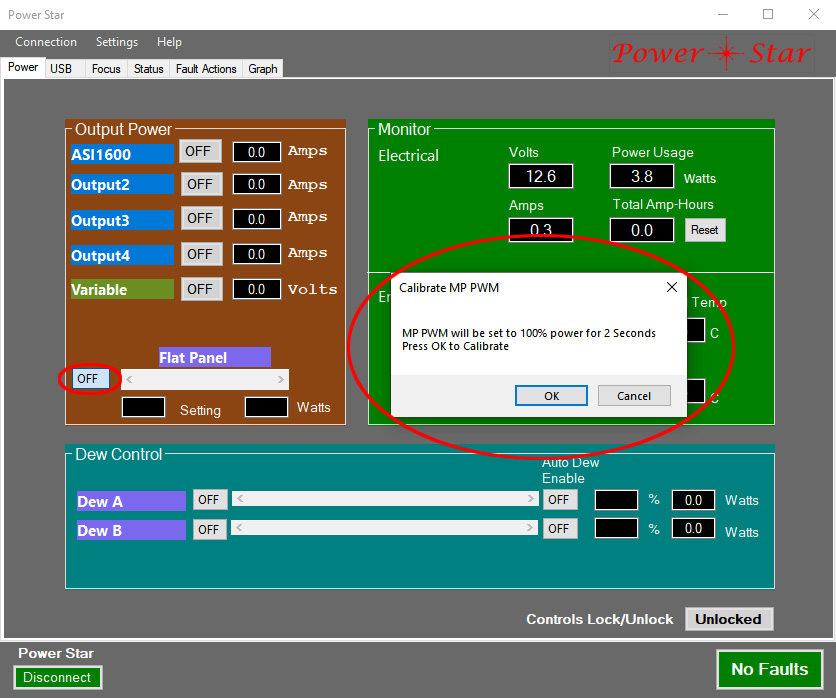
If the multi-purpose output is configured for PWM (sometimes referred to as “Fast PWM”), the current measurement system has a new problem to deal with: This PWM operates at 2kHz, which is much too fast to use the synchronous method used for dew channels. To work around this, the system attempts to measure the “full on” current, remember that value, and report the instantaneous current as the product of the remembered value and the slider position. The system will measure and remember the “full on” current any time the slider is set to the maximum position, but it also gives you the opportunity to perform this calibration when the PWM output is first turned on: A pop-up menu will appear asking whether it is OK to turn on the output for 2 seconds so it can make a measurement. The reason we ask if this is OK is that you may have connected a device that cannot tolerate the full 12V output for 2 seconds. For example, you could have a 5 volt fan (or other DC motor) that you operate by setting the PWM to about 425. For most DC motors this works great, but you need to be careful to not set the PWM slider too high, and must click “no” when prompted for the calibration. In this case you will not get an accurate current measurement for the PWM output.
Despite the poor accuracy of the per-port current measurement with low current flow, the system works quite well in distinguishing between “little current” and “no current”. When an output senses no current the displayed value (which, by definition, will be 0) will have a yellow background color to warn you that something may be wrong. For example, the device may have become disconnected. If the displayed value is 0 but the background is black there is a small current flow, but less than 0.1 amps. Where this doesn’t always work perfectly is that outputs 1 and 2 have a higher threshhold for the “no current” state because their maximum current capacity is much higher than the others (15 amps versus 6). A common example is when output 1 or 2 is used to power an astro camera that uses the 12V power only to operate the cooling in the camera. If cooling is turned off the current draw can be so low that it appears to be disconnected. In this case you can either move the camera’s 12V power to one of the other outputs, or simply ignore the warning. If you choose to ignore it, please confirm that the cooling is working correctly once enabled, either by the disappearance of the yellow background warning, or by the actual temperature report from the camera.
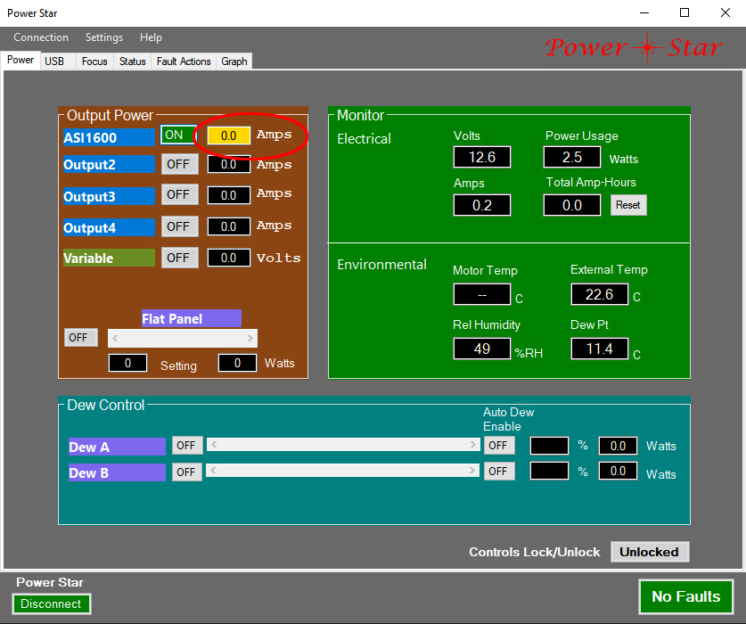
There is a small caveat related to the above discussion: When the multi-purpose output is configured for PWM operation the detection of “no current” is problematic because with the very rapid switching of the output on and off a bogus “no current” signal can appear as an over-current fault for the output. To avoid this, the multi-purpose output (only) has a small built-in load. Therefore, the “no current” warning does not work for this output, even when not configured for PWM mode. In the image above Output 1 (labeled as ASI1600) is showing the “no current” warning, but since this is one of the high capacity outputs it may be true that the camera is connected, but cooling is turned off. The imaging part of the camera is powered through its USB connection.
The Monitor section of the Power tab shows the instantaneous input voltage, total current, the corresponding wattage (volts times amps), and the accumulated amp-hours. All of these are quite accurate, although they are not updated frequently (every 5 seconds), so brief variations in voltage or current will not be obvious. The amp-hour gauge is useful for predicting battery life. If you reset the value (to zero) when a freshly charged battery is connected, and assuming you know the amp-hour capacity of the battery, this will tell you what portion of the capacity has been used. This is usually a more accurate method than simply watching the voltage decline as the battery discharges. Note that lead-acid batteries should not be allowed to discharge to less than half the rated capacity. Each type of battery chemistry is different, but other types, such as lithium-ion, are generally OK with much deeper discharge.
The Environment section shows the temperature, relative humidity, and dew point, all of which are self explanatory. In addition to the environment sensor data, if temperature data from a focus motor is available it is also displayed. These sensors may not agree with each other, even if the environment sensor is placed close to the focus motor. In general, I would trust the environment sensor more than the motor sensor. One could argue that the motor temperature is a better indication of the focuser temperature, since it is inside the motor housing, which is pretty well thermally coupled to the focuser. However, there are 2 things wrong with this argument: First, focus drift is not strictly related to the temperature of the focuser, but to the temperature of the telescope tube, since that is where most of the thermal expansion happens (assuming the tube is made of aluminum or steel). Second, the sensor inside the focus motor (motors from Optec and Starlight Instruments are supported) is affected by heat generated by the motor. Even when the motor is idle, a small current is used to hold the position (this is the Idle Current in the focuser configuration menu). This is why these manufacturers provide an “offset” parameter in their focuser apps – to compensate for the error.
Note that P*S does NOT support the temperature sensor used by Wa-chur-ed Observatory focus motors. This is simply because we didn’t want to use the code space needed to support it when Power*Star’s included environment sensor serves the same function (our sensor is NOT embedded in the motor).
The Graph tab shows the history of several key parameters; input voltage, total current, temperature, humidity, and dew point. It is often useful to examine these graphs to see what has happened over time. I don’t think I need to explain what the graphs mean, as it is pretty obvious. However, it should be noted that the graph lines are fitted to the samples, which means that the curves are generally smooth, even though changes can happen very quickly. The result is that the graph lines sometimes indicate some overshoot that did not really occur, and do not show some short-term changes.
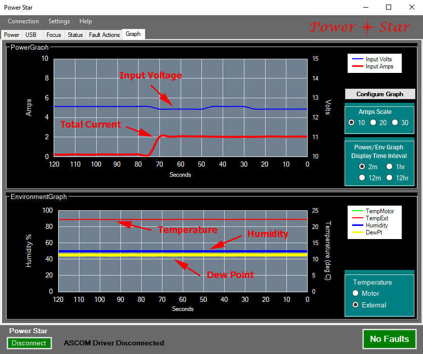
Note that you can select the time span of the displayed graph to be 2 minutes, 12 minutes, 1 hour, or 12 hours. The range for the environment parameters is automatically adjusted to suit the data, so pay attention to the vertical scale markings on the left and right side. They will not always be the same. The total current graph does not auto-scale, but you can manually choose a scale of 10, 20, or 30 amps.
The graph can be configured to determine colors, line styles, and line thickness. Of these, the only one that might need some explanation is the line thickness: Because multiple parameters are displayed in each graph, it is quite possible for graph lines to overlap. Unless you get into some very complicated color blending operations it can be difficult to distinguish one line from another. A simple solution to this problem is to use different line thicknesses. The lines are drawn in a sequence that follows how they are shown in the configuration menu. That is, the top parameters are drawn last, so overlay the lower ones. By making the upper lines thin and the lower lines thick, at least part of each line will always be visible, regardless of overlap. This is how the default thicknesses are arranged.
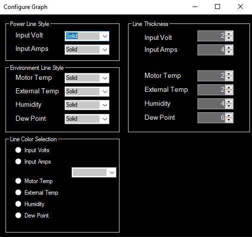
The default settings for graph configuration have been carefully chosen to maximize visibility and clarity under most circumstances, including the use of a red filter, so it is seldom necessary to make any changes here.